Use Python to analyse APT data in DASAPT

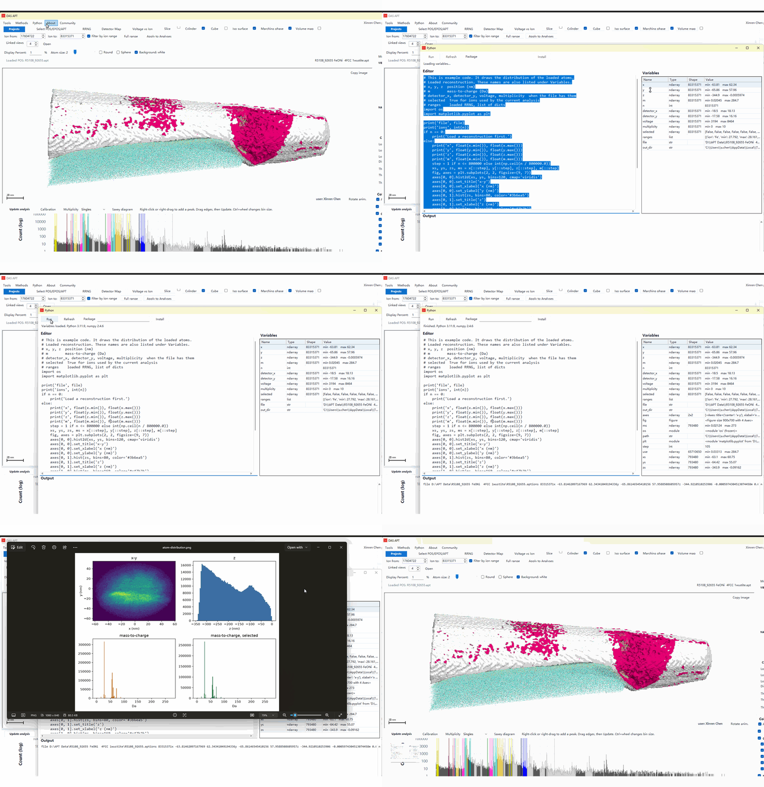
The Python window runs your own script on the reconstruction that is already open. DASAPT copies the ions into NumPy arrays, so the same positions, masses, and RRNG ranges you see in the 3D view are available under fixed names. NumPy is already imported as np.

Open it

1. Load a reconstruction (.pos, .epos, or .apt).
2. On the menu bar, click Python. The editor opens with an example, and the Variables table fills from the current file.
3. Click Run, or press Ctrl+Enter.
4. Click Refresh when you only want the variable list updated. Run already reads the reconstruction again, so a new ion range, cube, slice, or detector selection is included on the next run.

The status line reports the bundled Python and NumPy versions. In the recording that is Python 3.11.9 and NumPy 2.4.6.

Names already in the session

• x, y, z — position of every ion, in nm. These arrays are the whole file.
• m — mass-to-charge, in Da.
• n — number of ions. file — path of the loaded reconstruction.
• detector_x, detector_y, voltage, multiplicity — present when the file has them. A .pos file does not.
• selected — True for ions that pass the current ion-range, cube, slice, and detector filters. Use m[selected] (and the same index on x, y, z) to analyse that subset. The full arrays stay intact.
• ranges — the loaded RRNG, a list of dicts with ion, min, max, and color.
• out_dir — folder for files the script saves.

What the example draws

The script already in the editor prints the file and the ion count, then the min and max of x, y, z, and m. Above 800,000 ions it steps through the arrays so the figure stays small, and saves four panels to atom-distribution.png:

• x–y, a 2D histogram of the reconstruction cross-section.
• z, the depth histogram.
• mass-to-charge, every ion.
• mass-to-charge, selected, only ions that pass the current filter.

A line that starts with saved followed by a path opens that image. The example ends with print('saved', path), which is why the PNG appears after Run.

Install another package

Type a package name in Package, for example scikit-learn, and click Install. That runs pip inside the bundled environment. When it finishes, run the script again and import the package. Matplotlib is already there; the example uses it.

Python 窗口对当前已经打开的重构运行你自己的脚本。DASAPT 把离子放进 NumPy 数组，三维视图里的坐标、质量和 RRNG 范围都用固定的名字提供。NumPy 已经以 np 导入。

怎么打开

1. 载入重构（.pos、.epos 或 .apt）。
2. 在菜单栏点击 Python。编辑器里已有一段示例，Variables 表用当前文件填好。
3. 点击 Run，或按 Ctrl+Enter。
4. 只想更新变量表时点 Refresh。Run 会重新读取重构，所以下一次运行会带上新的离子范围、立方体、切片或探测器选择。

状态栏会写出内置的 Python 和 NumPy 版本。这段录屏里是 Python 3.11.9 和 NumPy 2.4.6。

会话里已有的名字

• x、y、z：每个离子的位置，单位 nm。这三个数组是整个文件。
• m：质荷比，单位 Da。
• n：离子个数。file：当前重构的路径。
• detector_x、detector_y、voltage、multiplicity：文件里有才提供。.pos 没有。
• selected：通过当前离子范围、立方体、切片和探测器过滤的离子为 True。用 m[selected]（x、y、z 用同一下标）分析这一部分。完整数组不会被改短。
• ranges：已载入的 RRNG，一列字典，含 ion、min、max、color。
• out_dir：脚本保存文件用的文件夹。

示例画了什么

编辑器里的脚本先打印文件名和离子数，再打印 x、y、z、m 的最小和最大值。离子超过 80 万时会按步长取样，避免图太大，然后把四张图存成 atom-distribution.png：

• x–y：重构截面的二维直方图。
• z：深度直方图。
• mass-to-charge：全部离子。
• mass-to-charge, selected：只保留通过当前过滤的离子。

以 saved 开头、后面跟路径的一行会打开那张图。示例最后是 print('saved', path)，所以 Run 之后 PNG 会弹出来。

再装一个包

在 Package 里输入包名，例如 scikit-learn，点 Install。这是在内置环境里运行 pip。装完后再运行脚本并导入。Matplotlib 已经在，示例用的就是它。