How to get very clear poles from your detector map

A hit-density map shows poles and zone lines only as a change in where the ions land. Lattice terraces on the tip change the local electric field. The gradient is strongest at a terrace edge, and that bends the ion trajectories. This local magnification shifts the hits on the detector, so the density follows the crystal projection. A pole is the centre of a terrace, not the edge itself. In the raw image that centre is often only a shallow low-density spot. In one example the density fell by about 15% across a pole, which is easy to miss. The maps below plot a crystallographic metric instead of hit density, following Breen et al., Ultramicroscopy 243 (2023) 113640.

SDM mapping

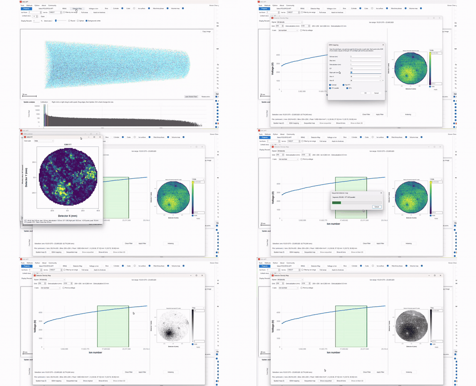
1. Open Detector Map. Drag the voltage window if you want only part of the evaporation.
2. Click SDM mapping.
3. Grid size is the square of ions used at each point (default 3 mm). Step is how far the next square moves (default 1 mm). Delocalization smooths the finished map (default 1 mm). The scan also runs one grid size past the outer hits.
4. ICF and flight path set the direction of Δ at that point. Defaults are 1.5 and 40 mm. LEAP 5000 XS on the other SDM dialog is ICF 2 and 100 mm.
5. Atom A and Atom B choose the pair. All and All uses every pair. A named pair uses only those two ions.
6. Contrast, Fast FFT, and Polynomial fit each open a map. Bright cells had enough ions (at least 40). Empty cells stay blank.

At each grid point DASAPT builds a spatial distribution map of the ions in that square, along the pole direction, inside a 1.5 nm ball. The in-depth resolution of a reconstruction is highest at a pole, because a pole is the centre of a lattice terrace and the evaporation sequence there is ordered. The SDM is then a histogram of the spacing along the plane normal, and that histogram carries a real lattice signal. Off the terrace the evaporation order is more random, the depth resolution is worse, and the SDM stays close to a smooth background.

Polynomial fit is the DF-fit score used for the spatial signal map in that paper. A quadratic is fit to the SDM and subtracted. The quadratic removes the background hump that comes from the edge of the local region, not the lattice peaks. The score is the remaining area, divided by the square of the number of ions:

E = (1/N²) ∫ [f(z) − f_fit(z)]² dz

On the same pole where the hit density changed by about 15%, this spatial signal rose by about 1000%. Fast FFT looks for one repeating spacing. Reconstructed plane spacing is not perfectly constant, so a single frequency is a less stable measure of that crystallinity than the polynomial-fit residual. Contrast is a separate score of how sharp the SDM peaks are.

Sequential evaporation mapping

1. On the same detector window, click Sequential map.
2. The ions are read in evaporation order. Each step takes a short segment. A grid is laid over the hits in that segment, and only the cell with the most hits is kept. It is kept only when that count reaches the density threshold.
3. The map is a histogram of those winning positions, not of the ions. Show sequential draws it in place of the hit density. A gray color scale makes the poles easy to see.

Evaporation at the centre of a lattice terrace is ordered, so successive hits land close together. Farther from that centre the order is more random and the hits spread out. A short segment therefore has one dense cell on the terrace centre and no such cell elsewhere. Keeping only that cell, and repeating it through the sequence, stacks the pole and leaves the rest of the detector dark. Breen et al. measured the same ordering as the lateral distance between successive hits, which is smaller on the pole. About 1–2 million ions from one grain is often enough; a much longer stretch can blur the pattern if the crystal or the evaporation field changes.

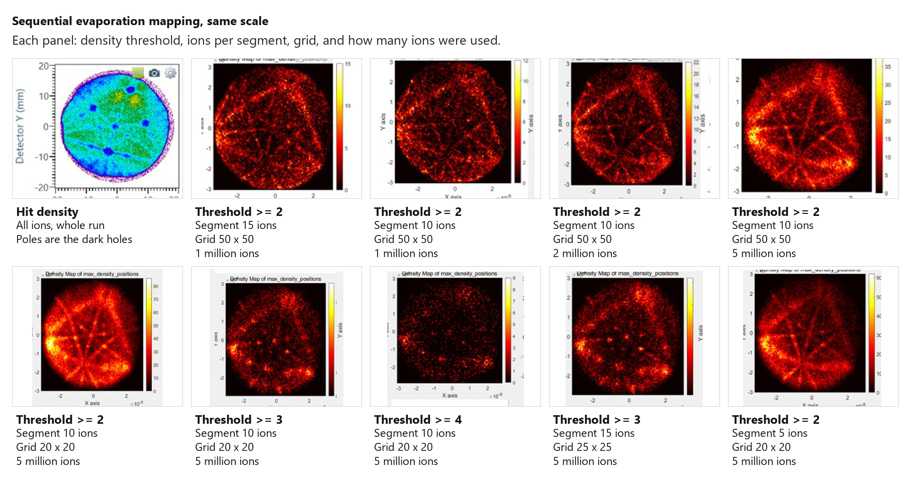
The label on the original plots was written as >2/10 50*50 1M. That is four numbers:

• Threshold (>2): the densest cell must contain at least this many hits, or that segment is dropped.
• Segment (10): how many ions are in one evaporation step.
• Grid (50×50): how the segment is divided.
• Ions (1M): how much of the sequence is included, here 1, 2, or 5 million.

Read across the figure, with every panel at the same size. At threshold 2, segment 10, and a 50×50 grid, going from 1 million to 5 million ions fills in the zone lines, because more segments vote for the same poles. At 5 million ions, a 20×20 grid is brighter than 50×50: each cell holds more ions, so the winning cell is more stable. Raising the threshold from 2 to 3 still shows the poles; threshold 4 rejects most segments and the map falls into sparse dots. A segment of 15 ions is smoother. A segment of 5 ions is grainier, because five ions barely locate a cell.

Reference

Breen, A.J., Day, A.C., Lim, B., Davids, W.J., Ringer, S.P. Revealing latent pole and zone line information in atom probe detector maps using crystallographically correlated metrics. Ultramicroscopy 243 (2023) 113640. https://doi.org/10.1016/j.ultramic.2022.113640